
의사결정 나무(Decision Tree)
의사결정 나무(Decision Tree)
가능한 대답이 두 가지인 이진 질의(Binary Question)의 분류 규칙을 바탕으로 최상위 루트 노드(Root Node)의 질의 결과에 따라 가지(Branch)를 타고 이동하며 최종적으로 분류 또는 예측값을 나타내는 리프(Leaf)까지 도달
- 범주형 자료 : Classification Tree(분류 나무)
- 수치형 자료 : Regression Tree(예측 나무)
Root Node : 최상위 노드
- Splitting : 하위 노드로 분리되는 것
- Branch : 노드들의 연결(의사결정나무의 일부분/Sub-Tree)
Decision Node : 2개의 하위 노드로 분리되는 노드
- Parent Node : 분리가 발생하는 노드
Leaf(Terminal Node) : 더 이상 분리되지 않는 최하위 노드
- Child Node : 분리가 발생한 후 하위 노드
규칙 기반으로 직관적으로 이해하기 쉽고 설명력이 좋은 알고리즘
- 각 노드 별로 불순도(Impurity)에 기반한 최적의 분류 규칙을 적용
- 분리(Splitting) 과정을 반복하면서 의사결정나무가 성장
- 각 리프(Leaf)는 동질성이 높은 적은 수의 데이터 포인트를 포함
동질성이 높은 그룹 구성을 위해 재귀적 파티셔닝(Recursive Partitioning) 수행
- 1단계 : 동질성이 높은 두 그룹으로 나눌 수 있는 이진 질의 적용
- 2단계 : 종료 조건을 만족할 때까지 1단계를 반복
1. 탐색적 데이터 분석
1-1. 빈도분석
DF.species.value_counts()setosa 50
versicolor 50
virginica 50
Name: species, dtype: int64
1-2. 분포 시각화
import matplotlib.pyplot as plt
import seaborn as sns

sns.pairplot(hue = 'species', data = DF)
plt.show()
2. Data Preprocessing
2-1. Data Set
X = DF[['sepal_length', 'sepal_width', 'petal_length', 'petal_width']]
y = DF['species']
2-2. Train & Test Split
from sklearn.model_selection import train_test_split

X_train, X_test, y_train, y_test = train_test_split(X, y,
                                                    test_size = 0.3,
                                                    random_state = 2045)

print('Train Data : ', X_train.shape, y_train.shape)
print('Test Data : ', X_test.shape, y_test.shape)
Train Data : (105, 4) (105,)
Test Data : (45, 4) (45,)
3. Modeling
3-1. Train_Data로 모델 생성
from sklearn.tree import DecisionTreeClassifier

Model_dt = DecisionTreeClassifier(random_state = 2045)
Model_dt.fit(X_train, y_train)
3-2. Visualization
from sklearn.tree import export_graphviz
import graphviz

graphviz.Source(export_graphviz(Model_dt,
                                class_names = (['setosa', 'virginica', 'versicolor']),
                                feature_names = (['sepal_length', 'sepal_width', 'petal_length', 'petal_width']),
                                filled = True))
3-3.Test_Data에 Model 적용
y_hat = Model_dt.predict(X_test)

y_hat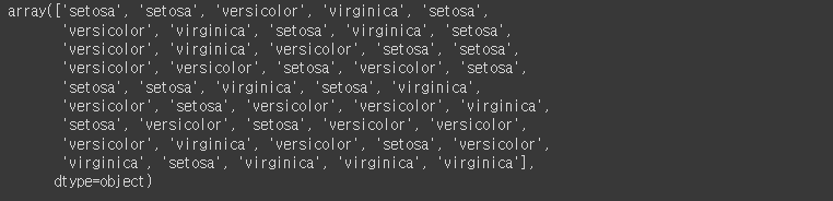
3-4. Confusion Matrix
from sklearn.metrics import confusion_matrix

confusion_matrix(y_test, y_hat)
3-5. Accuracy, Precision, Recall
from sklearn.metrics import accuracy_score, precision_score, recall_score

print(accuracy_score(y_test, y_hat))
print(precision_score(y_test, y_hat, average = None))
print(recall_score(y_test, y_hat, average = None))
3-6. F1_Score
from sklearn.metrics import f1_score

f1_score(y_test, y_hat, average = None)
array([1. , 0.93333333, 0.92307692])
4. 가지치기
- min_samples_split : 분할을 위한 최소한의 샘플데이터 개수
- min_samples_leaf : 말단 노드가 되기 위한 최소한의 샘플데이터 개수
- max_leaf_nodes : 말단 노드의 최대 개수
- max_depth : 트리모델의 최대 깊이를 지정
4-1. Model Pruning
from sklearn.tree import DecisionTreeClassifier

Model_pr = DecisionTreeClassifier(max_depth = 3,
                                  random_state = 2045)
Model_pr.fit(X_train, y_train)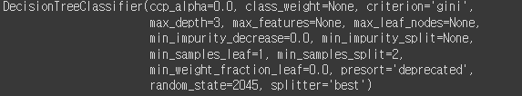
4-2. Model Visualization
from sklearn.tree import export_graphviz
import graphviz

graphviz.Source(export_graphviz(Model_pr,
                                class_names = (['setosa', 'virginica', 'versicolor']),
                                feature_names = (['sepal_length', 'sepal_width', 'petal_length', 'petal_width']),
                                filled = True))
4-3. Model Evaluate
#Confusion Matrix

from sklearn.metrics import confusion_matrix, accuracy_score, precision_score, recall_score

y_hat = Model_pr.predict(X_test)

print(confusion_matrix(y_test, y_hat))
print(accuracy_score(y_test, y_hat))
print(precision_score(y_test, y_hat, average = None))
print(recall_score(y_test, y_hat, average = None))
0.9555555555555556
[1. 0.875 1. ]
[1. 1. 0.85714286]
f1_score(y_test, y_hat, average = None)array([1. , 0.93333333, 0.92307692])
5. Feature Importance
5-1. Feature Importance 값 확인
Model_pr.feature_importances_plt.figure(figsize = (9, 6))
sns.barplot(Model_pr.feature_importances_,
['sepal_length', 'sepal_width', 'petal_length', 'petal_width'])
plt.show()