
인공지능/머신러닝
K-평균 군집(K-means Clustering) 1
2^7
2022. 6. 9. 16:39
K-means Clustering
입력값에 대한 출력값이 정해져 있지 않은 비지도학습 분석법
의사 중심점(Pseudo Center)을 각 군집 내 평균점으로 이동하며 반복
데이터 간 유사성(Similarity)을 계산하여 유사성이 높은 개체의 군집을 생성
여러 개의 군집(Cluster)를 생성하여 입력값이 속하는 그룹을 지정
동일한 그룹에 속하는 데이터는 유사성이 높고, 그룹 간에는 유사성이 낮음
K-means Clustering(K-평균 군집)
- 입력된 데이터를 K개의 군집(Cluster)로 묶는 분석방법
- 각 군집 내의 데이터들 간의 거리를 최소화
- 각 군집들 간의 거리를 최대화
- 각각의 데이터는 오직 한 개의 군집에만 포함됨
- 최초 K개의 의사 중심점(Pseudo Center)를 지정
- 분류된 데이터들의 평균점을 구하고 이동하는 과정을 반복
1. Import Packages and Lead Dataset
from sklearn.datasets import load_iris

iris = load_iris()- iris : Dictionary
- X : iris.data
- y : iris.target
DF = pd.DataFrame(data = iris.data,
                  columns = ['sepal_length',
                             'sepal_width',
                             'petal_length',
                             'petal_width'])

DF.head(3)
2. K-means Clustering
- n_clusters : 군집 개수 지정
- init : 초기 중심 설정 방식(기본값)
- max_iter : 최대 반복 횟수
2-1. Modeling
from sklearn.cluster import KMeans

kmeans_3 = KMeans(n_clusters = 3,
                  init ='k-means++',
                  max_iter = 15,
                  random_state = 2045)

kmeans_3.fit(DF)
2-2. Clustering Results
kmeans_3.n_iter_kmeans_3.cluster_centers_ #군집별 중심점kmeans_3.labels_ #군집 결과 레이블kmeans_3.inertia_78.85144142614601
3. Scree Plot
3-1. DataFrame
Z = pd.DataFrame(data = iris.data,
                 columns = ['sepal_length',
                            'sepal_width',
                            'petal_length',
                            'petal_width'])

Z.head(3)
3-2.K(1~9) 군집분석
inertia = []

K = range(1,10)

for k in K:
    kmeanModel = KMeans(n_clusters = k)
    kmeanModel.fit(Z)
    inertia.append(kmeanModel.inertia_)
3-3. 군집 중심까지의 제곱 거리의 합
inertia3-4. Plot the elbow
plt.figure(figsize = (9, 7))
plt.plot(K, inertia, 'bx-')
plt.xlabel('k')
plt.ylabel('inertia')
plt.title('Scree Plot with Kink')
plt.show()
4. Visualization with PCA(Principal Component Analysis)
4-1. target 및 cluster 추가
DF['cluster'] = kmeans_3.labels_
DF['target'] = iris.targetDF.head(3)4-2. 군집 결과 확인
DF.groupby('target')['cluster'].value_counts()4-3. PCA 차원 축소(4차원 -> 2차원)
from sklearn.decomposition import PCA

pca = PCA(n_components = 2)
pca_transformed = pca.fit_transform(iris.data)

pca_transformed[:5]
4-4. pca_x와 pca_y 추가
DF['pca_x'] = pca_transformed[:, 0]
DF['pca_y'] = pca_transformed[:, 1]DF.head(5)
4-5. 2차원 시각화
#군집 값 0, 1, 2 인덱스 추출

idx_0 = DF[DF['cluster'] == 0].index
idx_1 = DF[DF['cluster'] == 1].index
idx_2 = DF[DF['cluster'] == 2].index
idx_0, idx_1, idx_2
#0, 1, 2 인덱스 시각화

plt.figure(figsize = (9, 7))
plt.scatter(x = DF.loc[idx_0, 'pca_x'],
            y = DF.loc[idx_0, 'pca_y'],
            marker = 'o')
plt.scatter(x = DF.loc[idx_1, 'pca_x'],
            y = DF.loc[idx_1, 'pca_y'],
            marker = 's')
plt.scatter(x = DF.loc[idx_2, 'pca_x'],
            y = DF.loc[idx_2, 'pca_y'],
            marker = '^')

plt.xlabel('pca_x')
plt.ylabel('pca_y')
plt.title('Visualization by 2 PCA Components')
plt.show()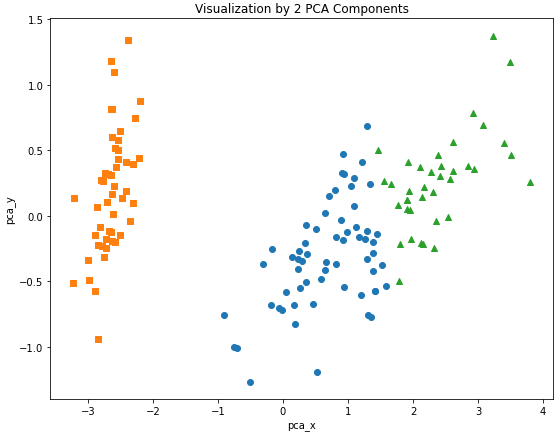
728x90