고정 헤더 영역

상세 컨텐츠
본문

1.Simple Linear Regression
1-1. 분석 변수 선택
DF1 = DF[['mpg', 'cylinders', 'displacement', 'weight']]

DF1.head(3)
1-2. 상관관계 그래프
# matplotlib

import matplotlib.pyplot as plt

plt.figure(figsize = (9, 6))
plt.scatter(x = DF1.weight, y = DF1.mpg, s = 30)
plt.show()
# seaborn
fig = plt.figure(figsize = (9, 6))
sns.regplot(x = 'weight', y = 'mpg', data = DF1, fit_reg = False)
plt.show()# pairplot
sns.pairplot(DF1)
plt.show()1-3.상관계수(Correlation Coefficient)
from scipy import stats

stats.pearsonr(DF1.mpg, DF1.weight)[0]
-0.831740933244335
from scipy import stats

stats.pearsonr(DF1.mpg, DF1.displacement)[0]
-0.8042028248058978
from scipy import stats

stats.pearsonr(DF1.mpg, DF1.cylinders)[0]
-0.7753962854205542
1-4.Train & Test Split
from sklearn.model_selection import train_test_split

X = DF1[['weight']]
y = DF1['mpg']

X_train, X_test, y_train, y_test = train_test_split(X, y,
                                                    test_size = 0.3,
                                                    random_state = 2045)

print('Train Data : ', X_train.shape, y_train.shape)
print('Test Data : ', X_test.shape, y_test.shape)
Train Data : (278, 1) (278,)
Test Data : (120, 1) (120,)
1-5.선형회귀 Modeling
from sklearn.linear_model import LinearRegression

RA = LinearRegression()
RA.fit(X_train, y_train)
LinearRegression(copy_X=True, fit_intercept=True, n_jobs=None, normalize=False)
print('weight(w) : ', RA.coef_)
print('bias(b) : ', RA.intercept_)
weight(w) : [-0.00766168]
bias(b) : 46.28223639092363
#결정계수(R-Sqaure)
RA.score(X_test, y_test)
0.7164499678296495
1-6. 모델 평가
from sklearn.metrics import mean_squared_error

y_hat = RA.predict(X_test)

mean_squared_error(y_test, y_hat)
17.01518447782976
1-7. Visualization
y_hat1 = RA.predict(X)

plt.figure(figsize = (9, 6))
ax1 = sns.distplot(y, hist = False, label = 'y')
ax2 = sns.distplot(y_hat1, hist = False, label='y_hat', ax = ax1)
plt.ylim(0, 0.07)
plt.show()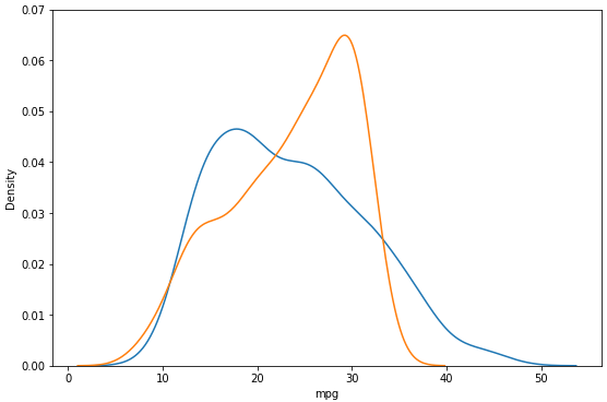
2. Lineare Regression
2-1. 분석 변수 선택
DF2 = DF[['mpg', 'cylinders', 'horsepower', 'weight']]

DF2.head(3)
2-2. Train & Test Split
from sklearn.model_selection import train_test_split

X = DF2[['weight']]
y = DF2['mpg']

X_train, X_test, y_train, y_test = train_test_split(X, y,
                                                    test_size = 0.3,
                                                    random_state = 2045)

print('Train Data : ', X_train.shape, y_train.shape)
print('Test Data : ', X_test.shape, y_test.shape)
Train Data : (278, 1) (278,)
Test Data : (120, 1) (120,)
2-3. 선형회귀 Modeling
from sklearn.preprocessing import PolynomialFeatures

poly = PolynomialFeatures(degree = 2, include_bias = False)
X_train_poly = poly.fit_transform(X_train)

print('변환 전 데이터: ', X_train.shape)
print('2차항 변환 데이터: ', X_train_poly.shape)
변환 전 데이터: (278, 1)
2차항 변환 데이터: (278, 2)
from sklearn.linear_model import LinearRegression

NL = LinearRegression()
NL.fit(X_train_poly, y_train)
LinearRegression(copy_X=True, fit_intercept=True, n_jobs=None, normalize=False)
# import numpy as np
# np.set_printoptions(suppress = True, precision = 10)

print('weight(w) : ', NL.coef_)
print('bias(b) : ', '%.8f' % NL.intercept_)
weight(w) : [-1.75042457e-02 1.53383105e-06]
bias(b) : 60.88867527
X_test_poly = poly.fit_transform(X_test)

NL.score(X_test_poly, y_test)
0.7525521808321769
2-4. 모델 평가
from sklearn.metrics import mean_squared_error

X_test_poly = poly.fit_transform(X_test)

mean_squared_error(y_test, NL.predict(X_test_poly))
14.848773810921921
2-5. Visualization
y_hat_test = NL.predict(X_test_poly)

plt.figure(figsize=(9, 6))
plt.plot(X_train, y_train, 'o', label = 'Train Data')
plt.plot(X_test, y_hat_test, 'r+', label = 'Predicted Value')
plt.legend(loc='best')
plt.xlabel('weight')
plt.ylabel('mpg')
plt.show()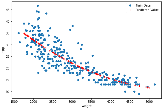
X_poly = poly.fit_transform(X)
y_hat2 = NL.predict(X_poly)

plt.figure(figsize = (9, 6))
ax1 = sns.distplot(y, hist=False, label="y")
ax2 = sns.distplot(y_hat2, hist=False, label="y_hat", ax=ax1)
plt.ylim(0, 0.07)
plt.show()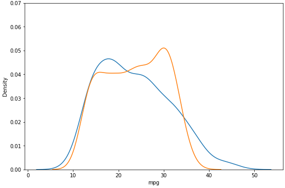
3. Multivariate Regression
3-1. 분석 변수 선택
DF3 = DF[['mpg', 'cylinders', 'displacement', 'weight']]

DF3.head(3)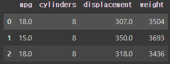
3-2. Train &Test Split
from sklearn.model_selection import train_test_split

X = DF3[['displacement', 'weight']]
y = DF3['mpg']

X_train, X_test, y_train, y_test = train_test_split(X, y,
                                                    test_size = 0.3,
                                                    random_state = 2045)

print('Train Data : ', X_train.shape, y_train.shape)
print('Test Data : ', X_test.shape, y_test.shape)
Train Data : (278, 2) (278,)
Test Data : (120, 2) (120,)
3-3. 다중회귀 Modeling
from sklearn.linear_model import LinearRegression

MR = LinearRegression()
MR.fit(X_train, y_train)
LinearRegression(copy_X=True, fit_intercept=True, n_jobs=None, normalize=False)
print('weight(w) : ', MR.coef_)
print('bias(b) : ', '%.8f' % MR.intercept_)
weight(w) : [-0.01766533 -0.00567273]
bias(b) : 43.74652237
MR.score(X_test, y_test)0.720971246285159
3-4. 모델 평가
from sklearn.metrics import mean_squared_error

mean_squared_error(y_test, MR.predict(X_test))
16.743872969214195
3-5. Visualization
y_hat3 = MR.predict(X_test)

plt.figure(figsize = (9, 6))
ax1 = sns.distplot(y_test, hist = False, label = 'y_test')
ax2 = sns.distplot(y_hat3, hist = False, label='y_hat', ax = ax1)
plt.ylim(0, 0.07)
plt.show()
4. 최종 시각화
y_hat3 = MR.predict(X_test)

plt.figure(figsize = (9, 6))
ax1 = sns.distplot(y_test, hist = False, label = 'y_test')
ax2 = sns.distplot(y_hat1, hist = False, label='y_hat', ax = ax1)
ax3 = sns.distplot(y_hat2, hist = False, label='y_hat', ax = ax1)
ax4 = sns.distplot(y_hat3, hist = False, label='y_hat', ax = ax1)
plt.ylim(0, 0.07)
plt.show()
728x90
'인공지능 > 머신러닝' 카테고리의 다른 글
| 회귀분석(Regression Analysis) 4 (0) | 2022.06.07 |
|---|---|
| 회귀분석(Regression Analysis) 3 (2) | 2022.06.07 |
| 회귀분석(Regression Analysis) 1 (1) | 2022.06.07 |
| Model Validation (0) | 2022.06.06 |
| 경사 하강법(Gradient Descent) (0) | 2022.06.06 |


