Fashion MNIST - Categorical Classification

Fashion MNIST - Categorical Classification

1.Fashion MNIST Data_Set Load & Review

1-1. Load Fashion MNIST Data_Set

from tensorflow.keras.datasets import fashion_mnist

(X_train, y_train), (X_test, y_test) = fashion_mnist.load_data()

#Train_Data Information

print(len(X_train))
print(X_train.shape)

print(len(y_train))
print(y_train[0:5])

#Test_Data Information

print(len(X_test))
print(X_test.shape)

print(len(y_test))
print(y_test[0:5])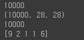

---

1-2. Visualization

import matplotlib.pyplot as plt

digit = X_train[0]
plt.imshow(digit, cmap = 'gray')
plt.show()

import numpy as np
np.set_printoptions(linewidth = 150)

print(X_train[0])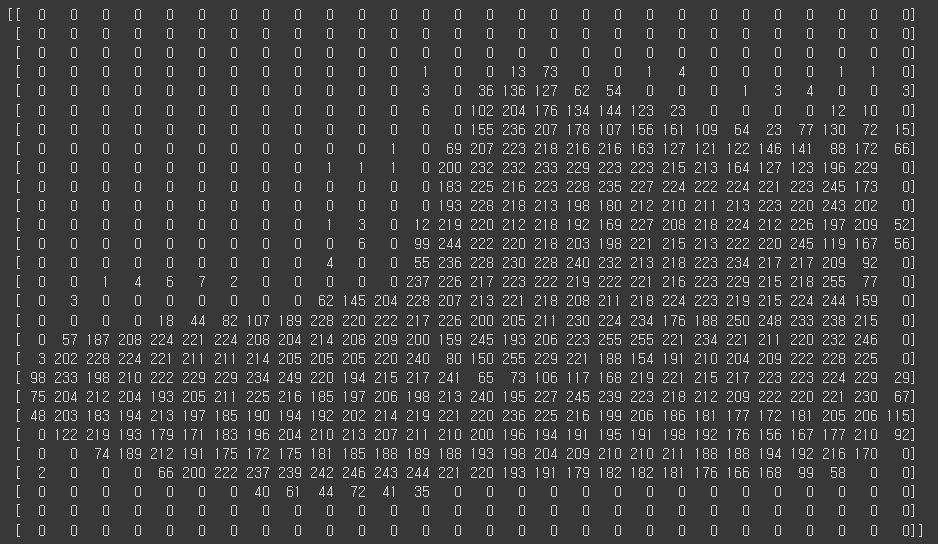

---

2. Data Preprocessing

2-1. Reshape and Normalization

X_train = X_train.reshape((60000, 28 * 28))
X_test = X_test.reshape((10000, 28 * 28))

X_train.shape, X_test.shape

((60000, 784), (10000, 784))

X_train = X_train.astype(float) / 255
X_test = X_test.astype(float) / 255

print(X_train[0])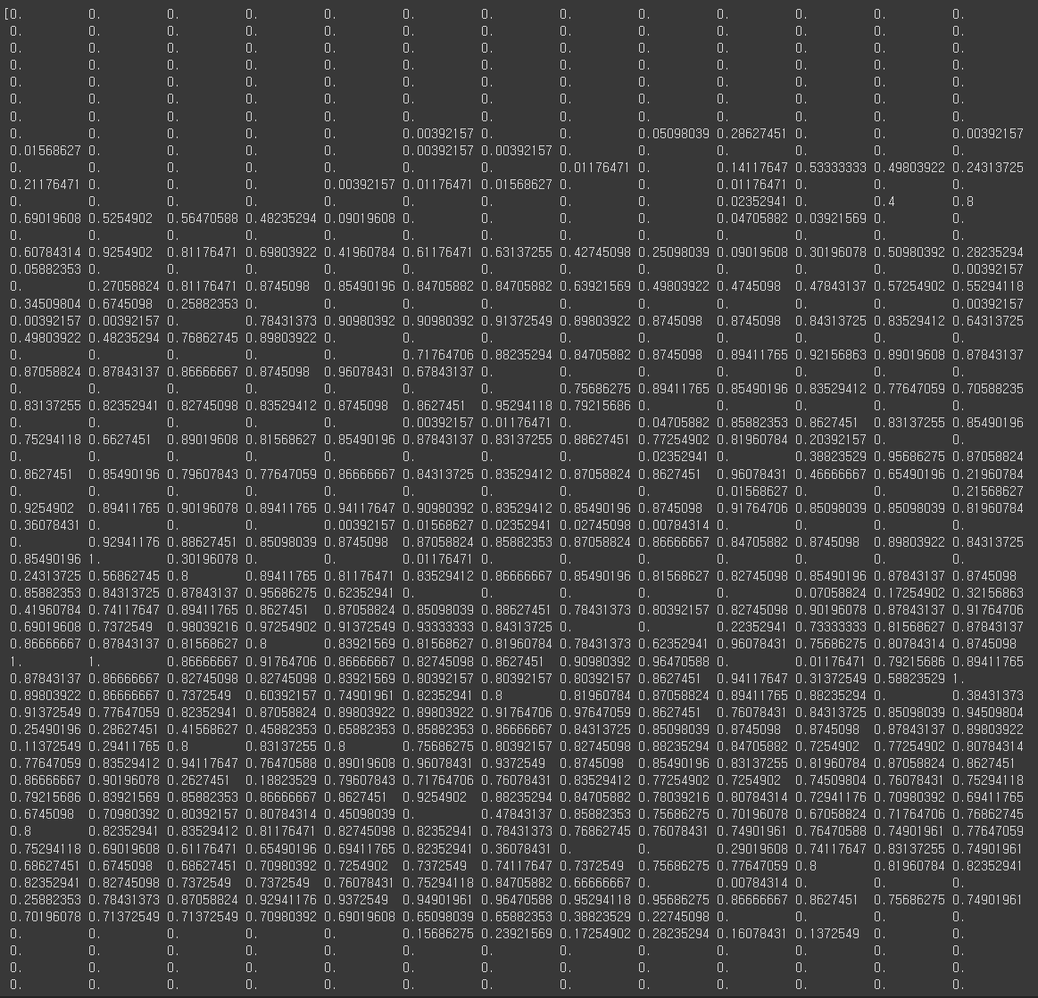

---

2-2.One Hot Encoding

from tensorflow.keras.utils import to_categorical

y_train = to_categorical(y_train)
y_test = to_categorical(y_test)

print(y_train[:5])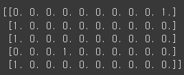

---

3.Keras Modeling

3-1. Model Define

from tensorflow.keras import models
from tensorflow.keras import layers

mnist = models.Sequential()
mnist.add(layers.Dense(512, activation = 'relu', input_shape = (28 * 28,)))
mnist.add(layers.Dense(256, activation = 'relu'))
mnist.add(layers.Dense(10, activation = 'softmax'))

mnist.summary()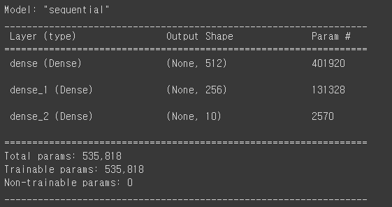

2개의 Hidden Layers & 768개의 Nodes

---

3-2. Model Compile

mnist.compile(loss = 'categorical_crossentropy',
              optimizer = 'rmsprop',
              metrics = ['accuracy'])

---

3-3. Model Fit

%%time

Hist_mnist = mnist.fit(X_train, y_train,
                       epochs = 100,
                       batch_size = 128,
                       validation_split = 0.2)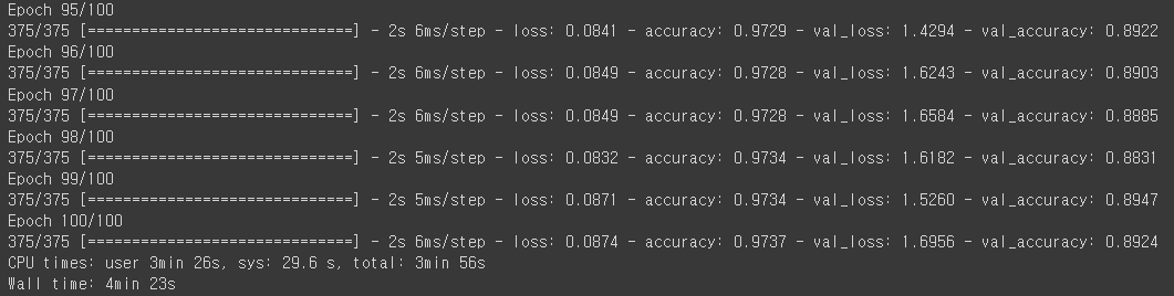

---

3-4. 학습 결과 시각화

import matplotlib.pyplot as plt

epochs = range(1, len(Hist_mnist.history['loss']) + 1)

plt.figure(figsize = (9, 6))
plt.plot(epochs, Hist_mnist.history['loss'])
plt.plot(epochs, Hist_mnist.history['val_loss'])
# plt.ylim(0, 0.25)
plt.title('Training & Validation Loss')
plt.xlabel('Epochs')
plt.ylabel('Loss')
plt.legend(['Training Loss', 'Validation Loss'])
plt.grid()
plt.show()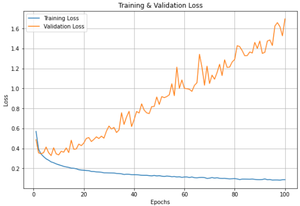

---

3-5. Model Evaluate

loss, accuracy = mnist.evaluate(X_test, y_test)

print('Loss = {:.5f}'.format(loss))
print('Accuracy = {:.5f}'.format(accuracy))

---

3-6. Model Predict

#Probability

np.set_printoptions(suppress = True, precision = 9)

print(mnist.predict(X_test[:1,:]))

[[0. 0. 0. 0. 0. 0. 0. 0. 0. 1.]]

print(np.argmax(mnist.predict(X_test[:1,:]), axis = 1))  #Class

[9]